# Review :Main idea of word2vec

• Start with random word vectors

• Iterate through each word in the whole corpus

• Try to predict surrounding words using word vectors :

  $$P(o|c)=\frac{\exp(u_{o}^{T}v_{c})}{\Sigma_{w\in V}\exp(u_{w}^{T}v_{c})}$$

• **Learning 😗*Update vectors so they can predict actual surroundings words better

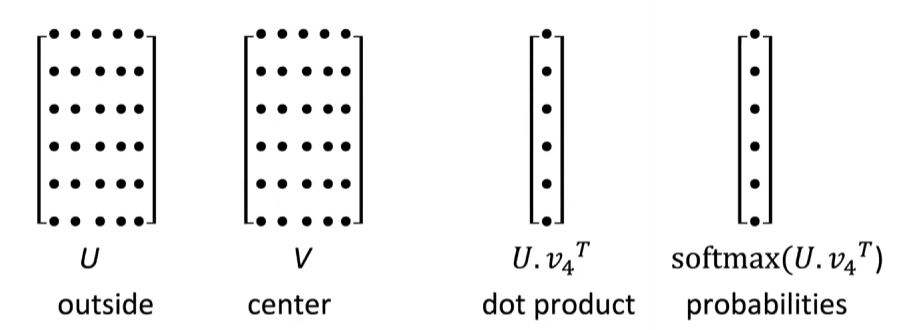
• Taking their dot product to get a probability to get a score of how likely a particular outside word is to occur with the center word.
• Then using the softmax transformation to convert those scores into probabilities.
• This model is what we call in NLP,a bag of words model,which don't actually pay any attention to word order or position. It doesn't matter if you're next to the center word or a bit further away on the left or right.The probability estimate would be the same.
• with this model we wanna to give reasonably high probabilities to the words that do occur in the context of the center word,at least if they do so at all often.
• Obviously lots of different words can occur,which means we more likely to talk about probabilities like 0.01 and numbers like that.
• Word2vec maximizes objective function by putting similar words nearby in space

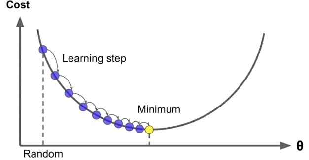
# Optimization : Gradient Descent

• To learn good word vectors: We have a cost function $\mathcal J(\theta)$ we want to minimize
• Gradient Descent is an algorithm to minimize $\mathcal J(\theta)$ by changing $\theta$
• Idea: from current value of $\theta $,calculate gradient of $\mathcal J(\theta)$,then take small step in the direction of negative gradient. Repreat

Update equation (in matrix notation)

$$\begin{aligned}\theta^{new}&=\theta^{old}-\alpha\nabla_\theta J(\theta)\\&\boxed{\alpha=step \ size \ or \ learning\ rate}\end{aligned}$$

# Update equation (for a single parameter)

$$\theta_j^{new}=\theta_j^{old}-\alpha\frac\partial{\partial\theta_j^{old}}J(\theta)$$

# code

1
2
3
4

while True:
    window = sample_window(corpus)
    theta_grad = evaluate_gradient(J,window,theta)
    theta = theta-alpha * theta_grad

# Stochastic gradients with word vectors (SGD)

• Iteratively (迭代地) take gradients at each such window for SGD
• But in each window, we only have at most $2m+1$ words,so $\nabla_\theta J_t(\theta)$ is very sparse (稀疏)!

$$\left.\nabla_\theta J_t(\theta)=\left[\begin{array}{l}0\\\vdots\\\nabla_{v_{like}}\\\vdots\\0\\\nabla_{u_I}\\\vdots\\\nabla_{u_{learning}}\end{array}\right.\right]\in\mathbb{R}^{2dV}$$

# Solution

• We might only update the word vectors that actually appear!
• either you need sparse matrix update operations to only update certain rows of full embedding matrices U and V,or you need to keep around a hash for word vectors
• Actually ,in PyTorch, word vectors are actually represented as row vectors.

$$\ \ \ \ \ \ d\\|V|\begin{bmatrix}\bullet&\bullet&\bullet&\bullet&\bullet\\\bullet&\bullet&\bullet&\bullet&\bullet\\\bullet&\bullet&\bullet&\bullet&\bullet\end{bmatrix}$$

# More details

# Why there are tow vectors?

center vector and the outside vectors

To make it much easier to optimization by average both at the end.

# Two model variants:

1. Skip-grams(SG)
   Predict context ("outside") words (position independent) given center word
2. Continuous Bag of Words (CBOW)
   Predict center word from (bag of) context words

# The skip-gram model with negative sample (HW2)

• The normalization term is computationally expensive
• $P(o|c)=\frac{\exp(u_o^Tv_c)}{\Sigma_{w\in V}\exp(u_w^Tv_c)}$
• Hence, in standard word2vec and HW2 we implement the skip-gram model with negative sampling
• So the idea of negative sampling is instead of using this softmax, we're going to train binary (二进制) logistic regression models for both the true pair of center word and the context word versus noise pairs

# Overall objective function(they maximize)

$$J(\theta)=\frac{1}{T}\sum_{t=1}^TJ_t(\theta) \\J_t(\theta)=\log\sigma\begin{pmatrix}u_o^Tv_c\end{pmatrix}+\sum_{i=1}^k\mathbb{E}_{j\sim P(w)}\begin{bmatrix}\log\sigma\begin{pmatrix}-u_j^Tv_c\end{pmatrix}\end{bmatrix}\\\sigma(x)=\frac1{1+e^{-x}}$$

$u_o$: This typically represents the output vector of a target word $o$. In the skip-gram model of Word2Vec, the target word is the word for which we are predicting the context words.

$u_j$: This represents the output vector of a context word $j$. In negative sampling, which is often used with Word2Vec,$ j$ can refer to a negative sample (a word that is not in the context of the target word).

$v_c$: This represents the input vector of a context word $c$. In the skip-gram model, context words are the words surrounding the target word within a specified window size.

$\log\sigma\begin{pmatrix}u_o^Tv_c\end{pmatrix}$:This term maximizes the probability of the context word$ c $given the target word $o$.

$\sum_{i=1}^k\mathbb{E}_{j\sim P(w)}\begin{bmatrix}\log\sigma\begin{pmatrix}-u_j^Tv_c\end{pmatrix}\end{bmatrix}$:This term deals with negative sampling. It minimizes the probability of randomly sampled words (negative samples) being in the context of the target word.

# The loss function notation more similar to class and HW2:

$$J_{neg-sample}(\boldsymbol{u}_{o},\boldsymbol{v}_{c},U)=-\log\sigma(\boldsymbol{u}_{o}^{T}\boldsymbol{v}_{c})-\sum_{k\in\{K sampled indices\}}\log\sigma(-\boldsymbol{u}_{k}^{T}\boldsymbol{v}_{c})$$

• We take $k$ negative samples (using word probabilities)
• Maximize probability that real outside word appears,
  minimize probability that random words appear around center word.
• Sample with $P(W)=\frac {U(W)^{\frac34}}Z$, the unigram distribution $U(w)$ raised to the $\frac 34$ power (We provide this function in the starter code).
• If you have a billion word corpus and a particular word occurred 90 times in it, you're taking 90 divided by billion.
• By taking threer-quarters ($\frac 34$) power, that has the effect if dampening the difference between common and rare words.

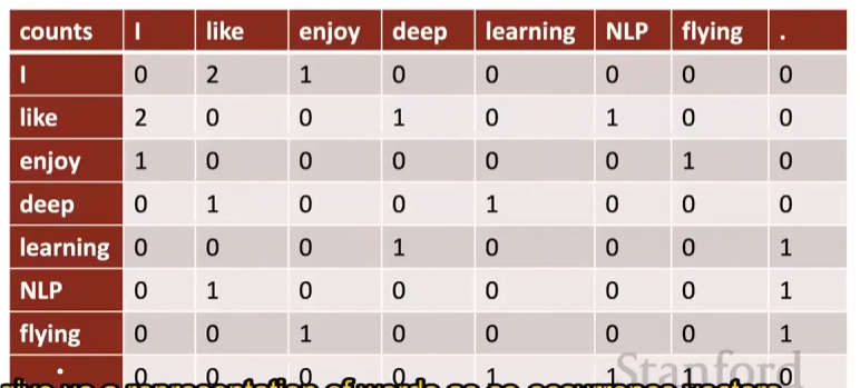
# Example : Window based co-occureence matrix

• Window length 1 (more common : 5-10)
• Symmetric (irrelevant whether left or right context)
• Example corpus:
  • I like deep learning
  • I like NLP
  • I enjoy flying
• To some extent that words have similar meaning and usage,so we expect them to have somewhat similar vectors.
• So if we had the word "you" as well on a larger corpus,we might expect "I" and "you" to have similar vectors because of "I like you like I enjoy you enjoy ".In this case, the sentences following "I" and "you" are the same.

# Co-occurrence vectors

• Simple count co-occurrence vectors
  • Vectors increase in size with vocabulary
  • Very high dimensional: require a lot of storage (though sparse)
  • Subsequent classification models have sparsity issues - Models are less robust
• Low-dimensional vectors
  • ldea: store “most" of the important information in a fixed, small number of dimensions: a dense vector
  • Usually 25-1000 dimensions, similar to word2vec
  • How to reduce the dimensionality?

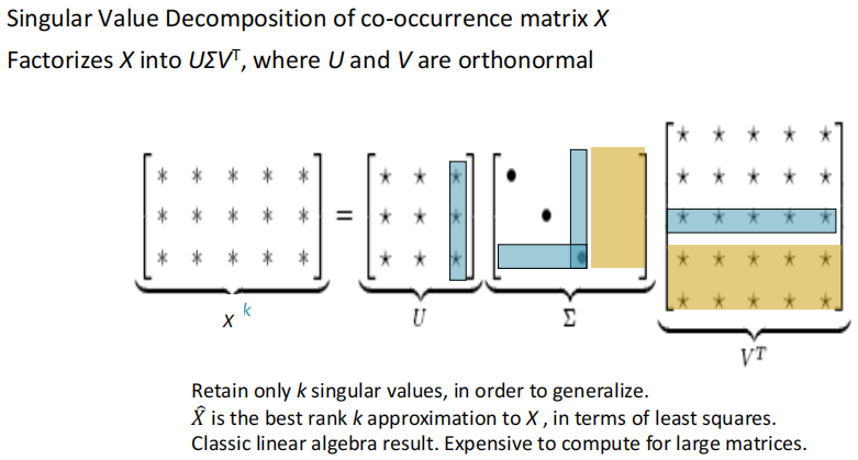
# Classic Method: Dimensionality Reduction on X(HW1)

# Some tips

# Scaling the counts in the cells can help a lot

Problem: function words (the, he, has) are too frequent àsyntax has too much impact. Some fixes:

• log the frequencies
• min(X, t), with t≈ 100
• Ignore the function words

# Ramped windows that count closer words more than further away words

# Use Pearson correlations instead of counts, then set negative values to 0

Crucial insight : Ratios of co-occurrence probabilities can encode meaning components

$$\begin{array}{c|c|c|c|c}&x=\text{solid}&x=\text{gas}&x=\text{water}&x=\text{random}\\\hline P(x|\text{ice})&\text{large}&\text{small}&\text{large}&\text{small}\\\hline P(x|\text{steam})&\text{small}&\text{large}&\text{large}&\text{small}\\\end{array}$$

# Question

How can we capture ratios of co-occurrence probabilities as linear meaning components in a word vector space?

# A:

Log-bilinear model: $w_i \dot w_j = log P(i|j)$

​ **with vector differences **: w_x \dot (w_a-w_b)=log \frac{P(x|a)}

# Intrinsic word vector evaluation

# Word Vector Analogies（类比）

$a:b::c?$

$man:woman::king$

$$\begin{array}{c}d=\arg\max_i\frac{\left(x_b-x_a+x_c\right)^Tx_i}{||x_b-x_a+x_c||}\\\end{array}$$

# Meaning similarity

Another intrinsic word vector evaluation

• Word vector distances and their correlation with human judgments
• Example dataset: WordSim353 http://www.cs.technion.ac.il/~gabr/resources/data/wordsim353/

# Extrinsic word vector evaluation

One example where good word vectors should help directly: named entity recognition: identifying references to a person, organization or location: Chris Manning lives in Palo Alto.

$$\begin{array}{|c|cccc|}\hline\text{Model}&\text{Dev}&\text{Test}&\text{ACE}&\text{MUC7}\\\hline\text{Discrete}&91.0&85.4&77.4&73.4\\\text{SVD}&90.8&85.7&77.3&73.7\\\text{SVD-S}&91.0&85.5&77.6&74.3\\\text{SVD-L}&90.5&84.8&73.6&71.5\\\text{HPCA}&92.6&\textbf{88.7}&81.7&80.7\\\text{HSMN}&90.5&85.7&78.7&74.7\\\text{CW}&92.2&87.4&81.7&80.2\\\text{CBOW}&93.1&88.2&82.2&81.1\\\text{GloVe}&\textbf{93.2}&88.3&\textbf{82.9}&\textbf{82.2}\\\hline\end{array}$$

$$w_i\cdot w_j=\log P(i|j)\\J=\sum_{i,j=1}^{V}f\left(X_{ij}\right)\left(w_{i}^{T}\tilde{w}_{j}+b_{i}+\tilde{b}_{j}-\log X_{ij}\right)^{2}$$

# Use word "bike" as an example

$$v_{\mathrm{pike}}=\alpha_{1}v_{\mathrm{pike}_{1}}+\alpha_{2}v_{\mathrm{pike}_{2}}+\alpha_{3}v_{\mathrm{pike}_{3},}\\\text{Where }\alpha_{1}=\frac{f_{1}}{f_{1}+f_{2}+f_{3}},\text{etc., for frequency}f$$