# MIXTURE OF WEAK & STRONG EXPERTS ON GRAPHS

# BACKGROUND

Propose a method for decoupling rich self-features of nodes and informative structures of neighborhoods by Mixture of weak and strong experts.

• weak expert: light-weight Multilayer Perceptron (MLP)
• strong expert: off-the-shelf GNN
• gating module: coordinated the collaboration between the two experts.
• confidence mechanism: base on the dispersion of the weak expert's prediction logits.

# OVERVIEW

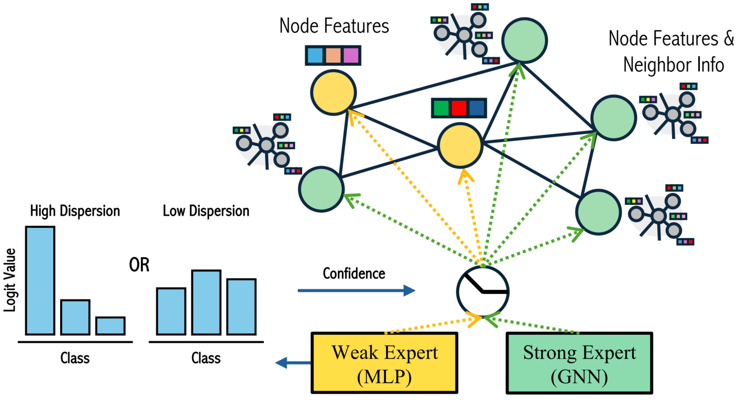
• Weak Expert (MLP): Handles node features independently without considering neighborhood information
• Strong Expert (GNN): Handles both node features and neighborhood information, making it useful for nodes that require relational data from surrounding nodes (such as heterophilous regions where the structure of the neighborhood is important).
• Gating Module: determining whether to use the weak expert (MLP) or the strong expert (GNN) for any given node——based on confidence score which is calculated from the dispersion(variation) of the MLP's output logits.
• the high Dispersion indicates low confidence from the weak expert, while the low Dispersion indicates high confidence from the weak expert.

# Methods

Use an intentionally imbalanced combination which mixed a simple Multi-Layer Perceptron (MLP) with an off-the-shelf GNN.

# Why MLP？

• Homophilous regions: nodes features are similar, which makes MLP who focused on the rich features of individual nodes more effective .
• Heterophilous regions: message passion could include noise, MLP expert can help "clean up" the dataset for the GNN, enabling the strong expert to focus on the more complicated nodes whose neighborhood structure provides useful information for the learning task.
• avoid oversmoothing and oversquashing

# Contributions

• use experts execute independent through their last layer and are then mixed based on a confidence score.
• score based on MLP's output, which made the system inherently biased.
• under the same training loss, the prediction of the GNN are more likely to be accept than MLP, due to the better generalization capability of GNN's.

# MOWST

# Algorithm

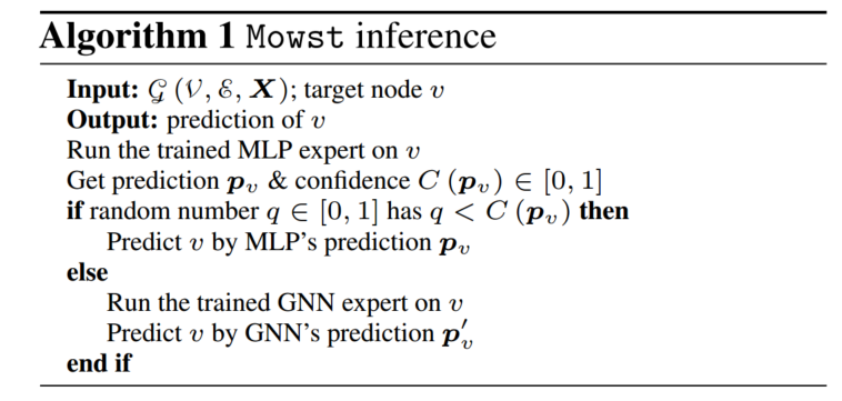
• Trained MLP expert used to make an initial prediction for node v to create the prediction $p_v$
• A confidence score $C(p_v)$ is computed which value between 0 and 1.
• Create a random number $q$ between 0 and 1. if $q$ is smaller than $C(p_v)$ then the system use MLP, on the contrast , it use GNN.

# Training

• $p_v$: the prediction of MLP

• ${p_v}'$: the prediction of GNN

• $L(p_v,y_v)$: the MLP incurs loss

• $C(p_v)$: the MLP occur probability

$$L_{\text{Mowst}} = \frac{1}{|\mathcal{V}|} \sum_{v \in \mathcal{V}} \left( C(p_v) \cdot L(p_v, y_v) + (1 - C(p_v)) \cdot L(p'_v, y_v) \right)$$

# INTERACTION BETWEEN EXPERTS

• divide the graph into m disjoint node partitions

• nodes are in the same partition $\mathcal M_i$ only if they have identical self-features. For all nodes in $mathcal M_i$. MLP generates the same prediction denoted as $\hat p_i$.

$$\{\hat{p}_i^*\} = \arg\min_{\{\hat{p}_i\}} L_{\text{Mowst}} = \arg\min_{\{\hat{p}_i\}} \sum_{1 \leq i \leq m} C(\hat{p}_i) \cdot \left( \hat{L}_{\alpha_i} (\hat{p}_i) - \mu_i \right)$$

• $$\mu_i = \frac{1}{|m_i|} \sum_{v \in m_i} L(p'_v, y_v)$$

  $\mu_i$ is the average loss of the fixed GNN on $\mathcal M_i$ nodes.

• $$\hat{L}_{\alpha_i}(\hat{p}_i) = \frac{1}{|m_i|} \sum_{v \in m_i} L(\hat{p}_i, \mathbf{y}_v) = -\sum_{1 \leq j \leq n} \alpha_{ij} \cdot \log \hat{p}_{ij}$$

  $\hat L_{\alpha_i}(\hat p_i)$ is the average MLP cross-entropy loss on nodes in $\mathcal M_i$

• for optimization problem $(2)$, the blow theorem quantifies its positions of the minimizer $\hat p_i ^*$ and the corresponding values of $C$

# Theorem

• continuous and quasiconvex: 连续的、拟凸的. monotonically non-decreasing: 单调非递减的

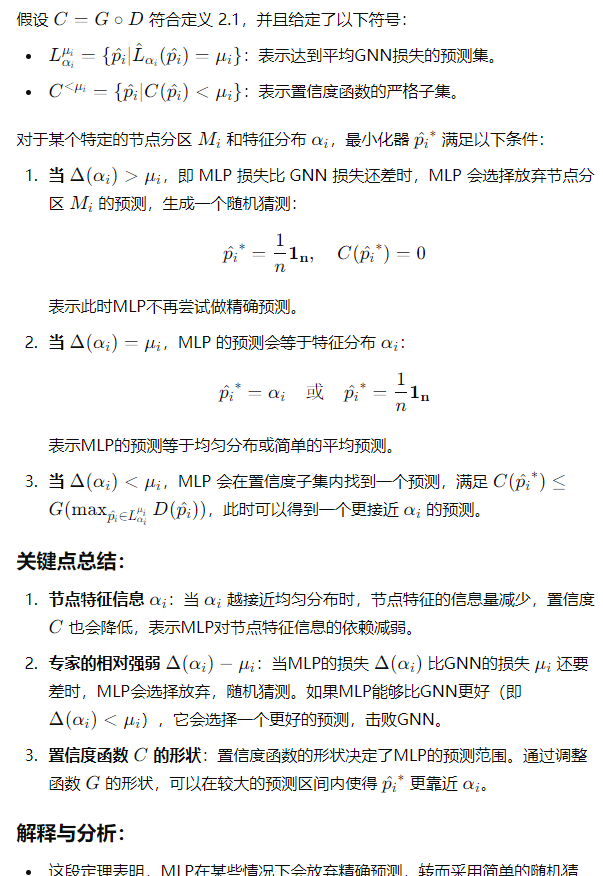
• $Δ\alpha $ reflects the best possible performance of any MLP on a group $\mathcal M_i$
• if $Δ\alpha < \mu_i$, which means MLP is better than GNN to process the special group, then MLP will choose $\hat p_i^*$ which closer to the features $\alpha_i$

• The expression $\frac{1}{n}$ 1 represents a vector where each element is$ \frac{1}{n}$
• **Node feature information $\alpha _i$ : **$\alpha _i$ being closer to $\frac{1}{n}$1 implies that node features are less informative. Thus confidence $C$ will be lower since it is harder to reduce the MLP loss
• Relative strength of experts, $Δ(\alpha_i)- \mu_i$: when the best possible MLP loss $Δ(\alpha_i)$ can't beat the GNN loss $\mu_i$, the MLP simply learns to give up on the node group $\mathcal m_i$ by generating random guess $\hat p_i^* = \frac{1}{n}1$. Otherwise the MLP will beat the GNN by learning a $\hat p_i^*$ in some neighborhood of $\alpha _i$ and obtaining positive $C$.
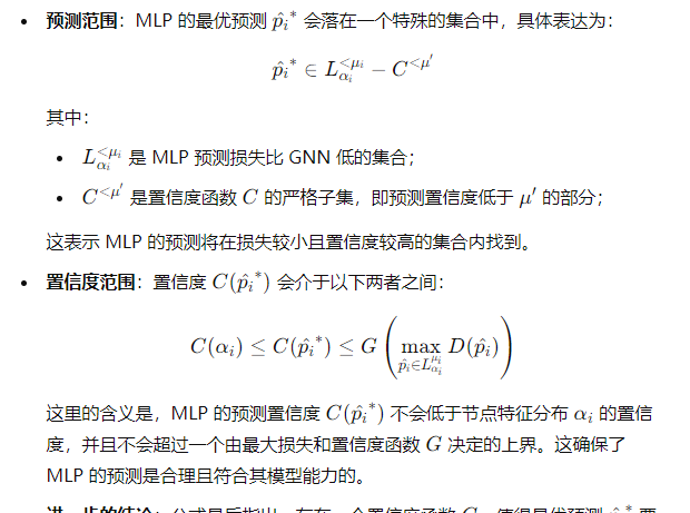
• Shape of the confidence function C: the sub-level set $\mathcal C^{< \mu ' }$ constrains the range of $\hat p_i^*$ .

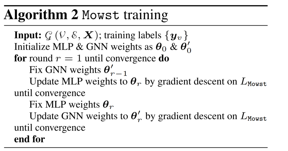
# Training

• compute the losses of the two experts separately, and then combine them via C to obtain the overrall loss L_
• use $C$ to combine the predictions of the two experts, $p_v$ and $p_v'$ and then calculate a single loss for $L_{Mowst}^*$

$$L^{\star}_{\text{Mowst}} = \frac{1}{|\mathcal{V}|} \sum_{v \in \mathcal{V}} L(C(p_v) \cdot p_v + (1 - C(p_v)) \cdot p'_v, y_v)$$

• assume that both experts have the same number of layers $\mathcal l$ and feature dimension $f$.

​

# 1. 研究背景与动机：

# 1.1. 知识图谱推理的现状：

• 关系路径推理方法：基于路径的方法（如随机游走和规则学习）在知识图谱推理中有较好的迁移性和可解释性，但它们的局限性在于只能捕获顺序连接的简单关系，难以处理复杂的局部子图结构。
• 图神经网络（GNN）方法：GNN 能够学习子图中的结构，但现有的 GNN 方法通常缺乏解释性，难以提供明确的推理证据。同时，GNN 在处理未见过的实体时表现有限，归纳能力不足。

# 1.2. 论文的动机：

现有的知识图谱推理方法在可解释性和复杂结构的捕捉方面各有不足。因此，作者希望设计一种新方法，既能够捕捉复杂的局部结构，又能够提供清晰的推理路径和解释性。

# 2. 挑战：

• 复杂结构的捕捉：现有基于路径的方法只能处理简单的顺序关系，无法有效捕捉局部子图中的复杂依赖关系。
• 高效推理：需要设计一种方法，能够在处理复杂图结构的同时，保持高效的推理计算。
• 可解释性：如何在推理过程中提供明确的局部证据和路径解释。

# 3. 方法：

# 关系有向图

• （r-digraph）是一种分层的有向图结构，源节点是查询实体$e_q$，目标节点是答案实体$e_a$。这个图结构通过保留多个重叠的关系路径来捕获知识图谱中的局部证据。该图的主要特点是层次化，每一层包含与上一层通过关系连接的节点，并且这些路径的长度不超过$L$
• 分层 ST - 图（Layered ST-graph）：一种有源节点和汇节点的有向图结构，其中的每条边都将相邻的两层节点连接起来。所有从$e_q$ 到$e_a$ 的路径都可以在途里表示出来。

# 构建

每一层的节点集 $V^\ell_{e_q, e_a|L}$ 表示在第 $\ell$ 层的节点，边集 $E^\ell_{e_q, e_a|L}$ 表示第 $ \ell$层的边。该图保留了从$ e_q$ 到 $e_a$ 之间的所有路径，并能表示复杂的子图结构。

# RED-GNN 模型

• 递归关系有向图编码：RED-GNN 通过动态编程方法，对共享边的多个 r-digraph 进行递归编码。该模型通过逐层收集从源节点开始的关系边，并递归构建出$L$ 层关系有向图。

• 消息传递机制：在每一层，RED-GNN 通过消息传递机制，聚合与实体 $ e_q$ 相关联的邻居节点的信息，生成新的节点表示。

  $$h_{e_o}^{\ell}(e_q, r_q) = \delta \left( W^{\ell} \cdot \sum_{(e_s, r, e_o) \in \tilde{\mathcal{E}}_{e_q}^{\ell}} \varphi \left( h_{e_s}^{\ell-1}(e_q, r_q), h_{r}^{\ell} \right) \right)$$

• 查询依赖的注意力机制：为了进一步提高推理的效果，RED-GNN 引入了注意力机制，该机制根据查询中的关系$r_q$，为不同的边分配不同的权重，聚焦于与查询相关的边。注意力机制通过计算注意力权重$\alpha$ 来控制边的重要性

$$\alpha_{e_s, r, e_o | r_q}^{\ell} = \sigma \left( \left( w_{\alpha}^{\ell} \right)^\top \text{ReLU} \left( W_{\alpha}^{\ell} \cdot \left( h_{e_s}^{\ell-1}(e_q, r_q) \oplus h_{r}^{\ell} \oplus h_{r_q}^{\ell} \right) \right) \right)$$

# 4. 实验与结果：

论文在多个数据集上对 RED-GNN 模型进行了实验评估，实验包括以下几部分：

• 归纳推理（Inductive Reasoning）：评估模型在未见过的实体和关系上的推理能力。结果表明，RED-GNN 在归纳推理任务上表现优越。
• 转导推理（Transductive Reasoning）：评估模型在已知的实体和关系上的推理表现。RED-GNN 在多个标准数据集上的准确率显著高于其他方法。
• 可解释性评估：RED-GNN 提供了可解释的推理路径，通过可视化模型推理出的路径，能够清楚地展示从源实体到目标实体的推理过程。

# 5. 总结：

# 5.1. 贡献：

• r-digraph 的引入：提出了 r-digraph 结构，能够捕捉复杂的局部证据，并保留了关系路径的解释性。
• RED-GNN 模型：提出了 RED-GNN 模型，通过递归的消息传递机制和查询依赖的注意力机制，实现了高效的推理和可解释性。
• 实验验证：在多个知识图谱数据集上的实验结果验证了 RED-GNN 模型的有效性和优越性。

# 5.2. 优势：

• 高效推理：RED-GNN 使用动态规划和递归消息传递，实现了在大规模知识图谱上的高效推理。
• 可解释性：通过构建 r-digraph 和查询依赖的注意力机制，模型在推理过程中保留了路径信息，提供了良好的可解释性。
• 强归纳能力：模型能够有效处理未见过的实体和关系，具备良好的归纳推理能力。

# 6. 总结阅读顺序：

1. train.py ：了解代码的整体结构和训练入口。
2. load_data.py ：理解数据的加载与处理流程。
3. base_model.py ：深入了解训练与评估的实现。
4. models.py ：理解 GNN 层和 RED-GNN 模型的结构与原理。
5. utils.py ：辅助工具函数，计算模型性能和选择 GPU